Pleasant Surprise
While trying to test the boundaries of what fastpages actually supports, I figured I’d try out installing and setting up an R Notebook as well. Luckily enough, it does indeed support compiling and building R kernels as well.
The first step will be to install an R kernel for the notebook which can be done using:
conda install -c r r-essentialsThis can be ran either from inside a notebook by prepending a ! in a cell such as !conda install -c r r-essentials or simply run it at the console if you’re in linux and in the project directory.
This is mostly an exibition post about how this can be done so we’re just going to show off some R stuff.
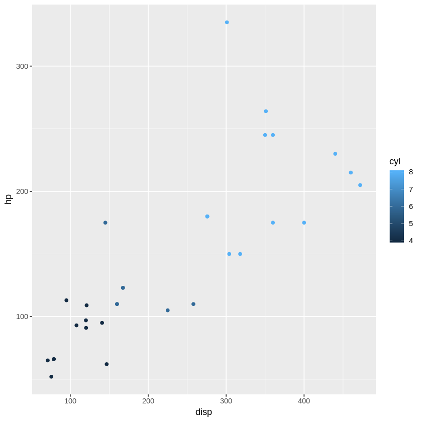
# I miss this selecting over Python's Pandas: order (mtcars$ gear, mtcars$ mpg), ]
Cadillac Fleetwood
10.4
8
472.0
205
2.93
5.250
17.98
0
0
3
4
Lincoln Continental
10.4
8
460.0
215
3.00
5.424
17.82
0
0
3
4
Camaro Z28
13.3
8
350.0
245
3.73
3.840
15.41
0
0
3
4
Duster 360
14.3
8
360.0
245
3.21
3.570
15.84
0
0
3
4
Chrysler Imperial
14.7
8
440.0
230
3.23
5.345
17.42
0
0
3
4
Merc 450SLC
15.2
8
275.8
180
3.07
3.780
18.00
0
0
3
3
AMC Javelin
15.2
8
304.0
150
3.15
3.435
17.30
0
0
3
2
Dodge Challenger
15.5
8
318.0
150
2.76
3.520
16.87
0
0
3
2
Merc 450SE
16.4
8
275.8
180
3.07
4.070
17.40
0
0
3
3
Merc 450SL
17.3
8
275.8
180
3.07
3.730
17.60
0
0
3
3
Valiant
18.1
6
225.0
105
2.76
3.460
20.22
1
0
3
1
Hornet Sportabout
18.7
8
360.0
175
3.15
3.440
17.02
0
0
3
2
Pontiac Firebird
19.2
8
400.0
175
3.08
3.845
17.05
0
0
3
2
Hornet 4 Drive
21.4
6
258.0
110
3.08
3.215
19.44
1
0
3
1
Toyota Corona
21.5
4
120.1
97
3.70
2.465
20.01
1
0
3
1
Merc 280C
17.8
6
167.6
123
3.92
3.440
18.90
1
0
4
4
Merc 280
19.2
6
167.6
123
3.92
3.440
18.30
1
0
4
4
Mazda RX4
21.0
6
160.0
110
3.90
2.620
16.46
0
1
4
4
Mazda RX4 Wag
21.0
6
160.0
110
3.90
2.875
17.02
0
1
4
4
Volvo 142E
21.4
4
121.0
109
4.11
2.780
18.60
1
1
4
2
Datsun 710
22.8
4
108.0
93
3.85
2.320
18.61
1
1
4
1
Merc 230
22.8
4
140.8
95
3.92
3.150
22.90
1
0
4
2
Merc 240D
24.4
4
146.7
62
3.69
3.190
20.00
1
0
4
2
Fiat X1-9
27.3
4
79.0
66
4.08
1.935
18.90
1
1
4
1
Honda Civic
30.4
4
75.7
52
4.93
1.615
18.52
1
1
4
2
Fiat 128
32.4
4
78.7
66
4.08
2.200
19.47
1
1
4
1
Toyota Corolla
33.9
4
71.1
65
4.22
1.835
19.90
1
1
4
1
Maserati Bora
15.0
8
301.0
335
3.54
3.570
14.60
0
1
5
8
Ford Pantera L
15.8
8
351.0
264
4.22
3.170
14.50
0
1
5
4
Ferrari Dino
19.7
6
145.0
175
3.62
2.770
15.50
0
1
5
6
Porsche 914-2
26.0
4
120.3
91
4.43
2.140
16.70
0
1
5
2
Lotus Europa
30.4
4
95.1
113
3.77
1.513
16.90
1
1
5
2
order (mtcars$ gear, mtcars$ mpg), ] %>% ggplot (aes (disp, hp, colour = cyl)) + geom_point ()
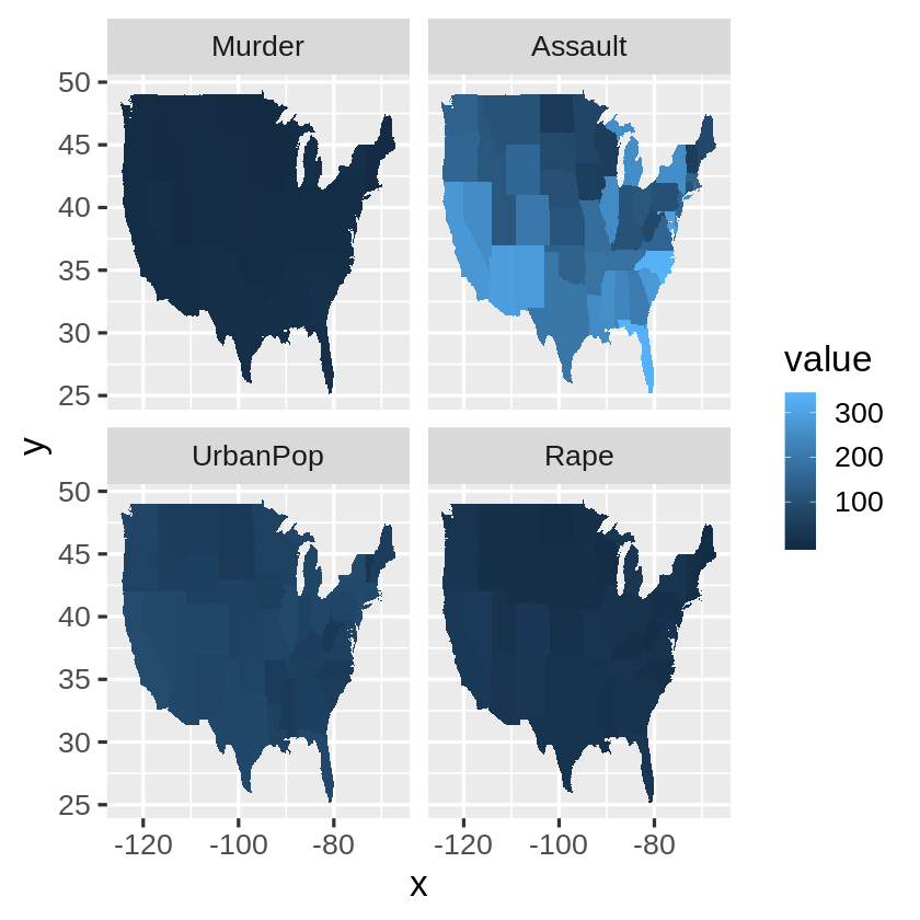
<- data.frame (state = tolower (rownames (USArrests)), USArrests)# Equivalent to crimes %>% tidyr::pivot_longer(Murder:Rape) <- lapply (names (crimes)[- 1 ], function (j) {data.frame (state = crimes$ state, variable = j, value = crimes[[j]])<- do.call ("rbind" , vars)<- map_data ("state" )ggplot (crimes_long, aes (map_id = state)) + geom_map (aes (fill = value), map = states_map) + expand_limits (x = states_map$ long, y = states_map$ lat) + facet_wrap ( ~ variable)
I did also try to use ggvis as well but it just wont display properly so that’s unfortunately out.