What is the Chi-Squared Test?

The purpose of the Pearson Chi-Squared Test is to determine whether the observed data is different than what would be expected. You can see this quite clearly from the actual formula being used; This is one of those moments where the description is less elegant that simply looking at the math: \[ \sum\frac{(Observed - Expected)^2}{(Expected)} \]

This is very commonly used in A/B Testing since the purpose is to test for independence of the different categories. If you’re not familiar with the term, then an A/B Test is when you’re running an experiment and you’re attempting to determine whether changing some specific interaction affects how people use a product. Common examples would be changes in appearance or behavior of buttons on websites and you’ve likely been subjected to this - whether you knew or not.

Chi-Squared Test in R

Since I am more familiar with doing this in R than in Python we’ll start here. Thankfully, R has this included by default with little to no requirements. I’m including the tidyverse since the tooling is superior to Base R but it wont have anything to do with the actual test itself.

We’ll need some data and thankfully I’ve ferreted this away from an online class I’ve taken previously. It’s stored on a site called Data.World. You are welcome to use this link if you like but it might not work in the future since I’m considering moving the data off the platform and somewhere else.

library(tidyverse)

── Attaching packages ─────────────────────────────────────── tidyverse 1.3.2 ──
✔ ggplot2 3.4.0      ✔ purrr   1.0.1 
✔ tibble  3.1.8      ✔ dplyr   1.0.10
✔ tidyr   1.3.0      ✔ stringr 1.5.0 
✔ readr   2.1.3      ✔ forcats 0.5.2 
── Conflicts ────────────────────────────────────────── tidyverse_conflicts() ──
✖ dplyr::filter() masks stats::filter()
✖ dplyr::lag()    masks stats::lag()

df = read_csv(
    "https://query.data.world/s/ccu3fx6fivcq2vdyavd26fhzk5tokq",
    col_types='if' # specify the column types are integer, factor.
)
df

# A tibble: 60 × 2
   Subject Pref 
     <int> <fct>
 1       1 B    
 2       2 B    
 3       3 B    
 4       4 B    
 5       5 B    
 6       6 B    
 7       7 B    
 8       8 B    
 9       9 A    
10      10 A    
# … with 50 more rows

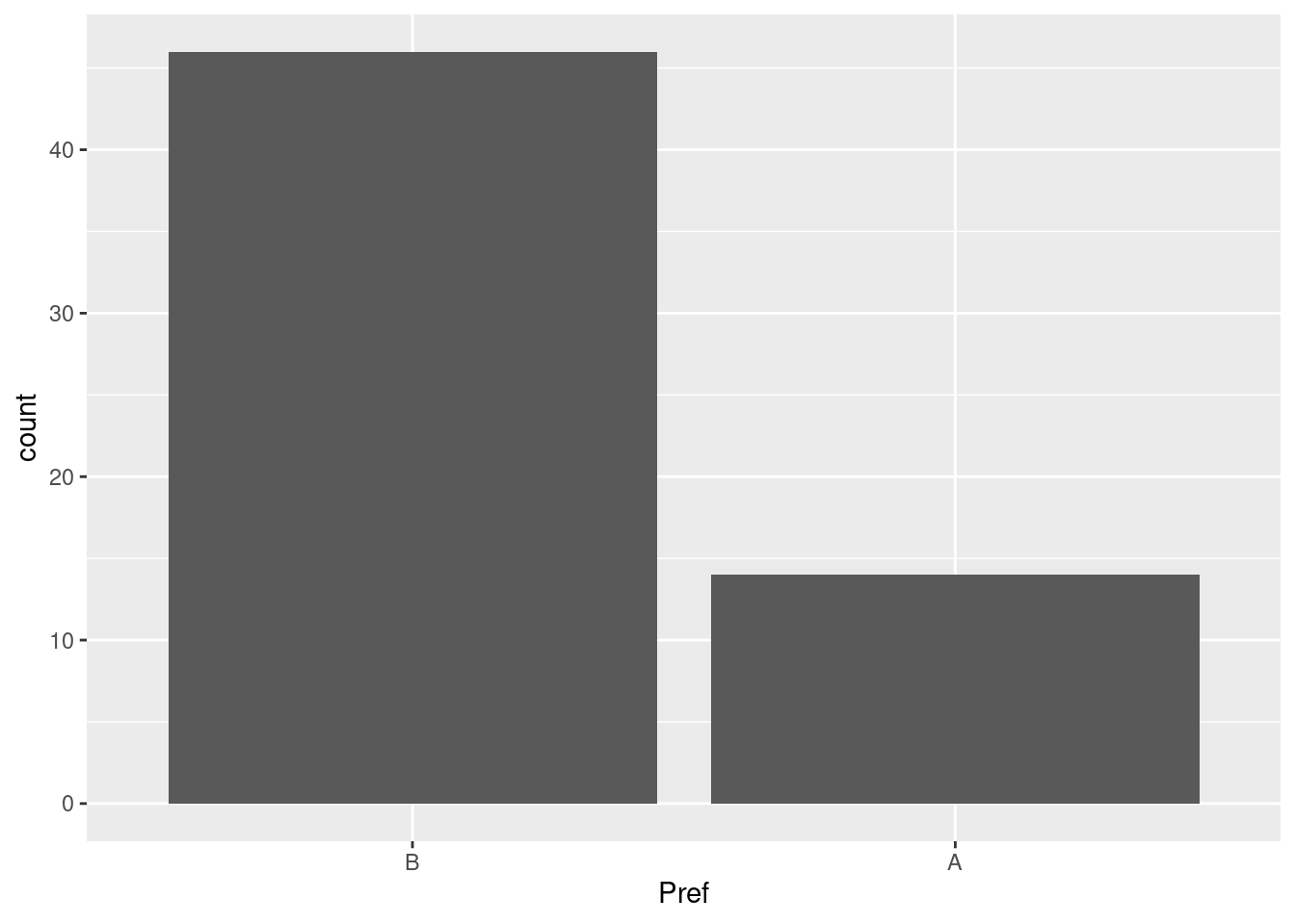
Looking at the data collect, we can see that we would in fact expect there to be a difference in the categories; it’s pretty obvious from the graph that they’re different by quite a bit:

df %>%
    ggplot(aes(x=Pref)) +
    geom_bar()

The function chisq.test() expects the class to be of type table so we cannot quite dump anything into it. We’ll need to first format the input how it expects using the function xtabs() and the formuala notation. With the maggitr package, you can emulate the pipe operator like in bash and it makes reading R code so much nicer:

# take the data
df %>%
    # format it as expected
    xtabs(~ Pref, .) %>%
    # pipe into the test for the results.
    chisq.test


    Chi-squared test for given probabilities

data:  .
X-squared = 17.067, df = 1, p-value = 3.609e-05

A reminder that your category will need to be a factor otherwise you’re get an error here. Looking at the results, it is what we expected - namely that the two are not independent and therefore we’d reject the null hypothesis of independence. For us, this is what we want because it means that there is a difference relationship between the two categories.

Chi-Squared Test in Python

For python, we’ll need the wonderful scipy package which you can get via python3 -m pip install scipy. Doing this in python turns out to be a bit tricky and not as straight forward. What we’ll need to do is make a pivot table aggregating on the length of the index. The .T in pandas just does a transpose and sometimes I do this for readability purposes:

import pandas as pd
import scipy as sp

df = pd.read_csv('https://query.data.world/s/rqmmkifx4fo2uaymurkmb4ibcu25p4')
props = df.pivot_table( index = 'Pref', aggfunc=len).T
props

Pref      A   B
Subject  14  46

Ok, now we’ll run the test and compare this against our results with R:

# Chi-Square test; don't do the pivot else it fails:
result = sp.stats.chisquare(
    df.pivot_table(
        index = 'Pref', aggfunc=len
    )
)

# Chi Statistic, P value
print((
    f"The Chi-Squared statistic is {round(result.statistic[0],2)}\
    and the p-value is {result.pvalue[0]:.3E}."))

The Chi-Squared statistic is 17.07    and the p-value is 3.609E-05.

Exactly as expected!

Thoughts

If you’re doing experiments then you’re going to be using this often. And, I would recommend using my method here. I found some examples of other people’s solutions and mine is both the cleanest and simplest way to do this. There were some uses of pd.crosstab() - which is neat - but even the documentation states that it’s front end for pivot_table() anyways and I found it really annoying trying to get to work with this example. Hopefully this makes your life easier while working on A/B Testing.